Yet Another Generative Adversarial Network (GAN) Guide in Keras, with MNIST testing example

Generative Adversarial Network (GAN) is a brilliant idea. By combining the power of generative model and a classifier and training them against each other, GAN can eventually generate samples that could fool classifier and even human.

We can start coding by writing a simple generator. It takes noises as input and returns a picture, which is of size 28*28*1 in MNIST. The noise could be of any size theoretically; however, if the dimension of noises is too small, the generating power is obviously lacking (imaging the generator with 1-dimension noise input). Say the noise input is of 32 dimensions, and for each dimension, a noise input is sampled uniformly from -1 to 1. For the next few layers, we reshape the noise to the size of 7*7*(*), then upsample it until we have an output of size 28*28*(*), and finally compress the output into 28*28*1 and add an activation function of ‘tanh’ in order to return an image of range [-1, 1] in each pixel. A simplified version of generator (with 4 layers that convert [64] -> [7*7*128] -> [14*14*64] -> [28*28*32] -> [28*28*1]) looks like this:

    # 64 -> 7*7*128 -> 14*14*64 -> 28*28*32 -> 28*28*1
    # Specify the shape of output for generator
    height = 28
    width = 28
    scale = 4
    init_shape = (int(np.ceil(width / scale)),
                  int(np.ceil(height / scale)),
                  32 * scale)

    # Noise dimension is 64
    entrance = Input((64,))
    temp = entrance

    # Dense layer and reshape for image generation
    temp = Dense(np.prod(init_shape))(temp)
    temp = BatchNormalization(momentum=batch_norm_momentum)(temp)
    temp = LeakyReLU(alpha=relu_alpha)(temp)
    temp = Reshape(init_shape)(temp)
    temp = Dropout(dropout)(temp)

    # Use UpSampling2D and Conv2D for up sampling
    for layer in range(2):
        temp = UpSampling2D()(temp)
        temp = Conv2D(
            filters=32 * 2 ** (1 - layer),
            kernel_size=5,
            strides=1,
            padding='same')(temp)
        if batch_norm:
            temp = BatchNormalization(momentum=batch_norm_momentum)(temp)
        temp = LeakyReLU(alpha=relu_alpha)(temp)
        temp = Dropout(dropout)(temp)

    # Compress the layers into output shape
    temp = Conv2D(
        filters=1,
        kernel_size=5,
        strides=1,
        padding='same')(temp)

    temp = Activation('tanh')(temp)
    generator = Model(entrance, temp)

Now we are done the generator, the discriminator (classifier that differentiates generated images from the real ones) should be even easier.  It takes a 28*28*1 image and gives out a probability of the input being real ([28*28*1] -> [14*14*64] -> [7*7*128] -> [4*4*256] ->[4096] ->[1]). Note that the discriminator should not be too powerful, otherwise it will simply crush the generator before it even begins to learn, which results in an early failure.

    entrance = Input((28, 28, 1))
    temp = entrance

    # Alternatively, could use average pooling for down sampling
    for layer in range(3):
        temp = Conv2D(
            filters=64 * 2 ** layer,
            kernel_size=5,
            strides=2,
            padding='same')(temp)
        if batch_norm:
            temp = BatchNormalization(momentum=batch_norm_momentum)(temp)
        temp = LeakyReLU(alpha=relu_alpha)(temp)
        temp = Dropout(dropout)(temp)

    # Flatten the convolutional net and use sigmiod to classify the input
    temp = Flatten()(temp)
    temp = Dense(1, activation='sigmoid')(temp)
    discriminator = Model(entrance, temp)

Before we head to the training, we need the discriminator model and adversarial model ready. The first one is simply our discriminator, trained with the loss function of binary cross entropy; and the second one is built by stacking generator and discriminator together, with the weights of discriminator frozen. This is because during the training of generator, we are going to feed adversarial model with fake images and real labels, and we do not want to mess up the discriminator in this phase. The code looks like this:

# Build discriminator_model
self.dm = Sequential([self._discriminator])
self.dm.compile(
    loss='binary_crossentropy',
    optimizer=Adam(lr=0.0002, decay=1e-06),
    metrics=['accuracy'])

# Build adversarial_model:
self._discriminator.trainable = False
self.am = Sequential([self._generator, self._discriminator])
self.am.compile(
    loss='binary_crossentropy',
    optimizer=Adam(lr=0.0001, decay=1e-06),
    metrics=['accuracy'])

Now we have both models ready, let’s proceed to the training part. For each epoch, we are going to feed the discriminator a bunch of real images from MNIST, and then a bunch of fake ones from our currently crapy generator (with labels 1 and 0 separately). I have not tested too much on this part yet, but I have heard that mixing real and fake samples could be bad for the discriminator. The training of discriminator looks like this:

# Select a random half batch of images
indices = np.random.randint(
    0, training_sample_num, half_batch_size)
half_batch_samples = self._training_samples[indices]

# Generate a half batch of fake images from noise
half_batch_noise = self.get_noise(half_batch_size)
half_batch_mimics = self._generator.predict(half_batch_noise)

# Train the discriminator model wih half real and half fake samples
# Do not mix the real images with the fake ones
d_loss_samples = self.dm.train_on_batch(
    half_batch_samples, np.ones((half_batch_size, 1)))
d_loss_mimics = self.dm.train_on_batch(
    half_batch_mimics, np.zeros((half_batch_size, 1)))
d_loss = np.add(d_loss_samples, d_loss_mimics) / 2

And in the same epoch, we would like to train the adversarial model with generated images along with the real labels, which can make our generator return more realistic images in the eyes of the discriminator, and the code is even simpler:

batch_noise = self.get_noise(batch_size)
g_loss = self.am.train_on_batch(
    batch_noise, np.ones((batch_size, 1)))

That’s pretty much all the things we need to do for a GAN to be trained with MNIST. Finally, we can pick a number and feed it into GAN. Let’s pick number ‘5’ from MNIST for its non-symmetrical appearance, and use here are the results:

These three images are obtained with uniform noise and looks… okay I guess. And here are some results using noise with Wigner semicircle distribution:

And digits definitely look clearer and more realistic. I think Gaussian noise will also work well this GAN in this case. Feel free to check out all the code, including some potential optimization at CycleGAN.

Paper Review: Low Latency Analytics of Geo-distributed Data in the Wide Area

Summary:

Iridium is system build for low-latency queries in widely distributed datacenter scenario. In this case the latency is primarily caused by bandwidth limitation during intermediate data transfer. Iridium counters the problem by relocating the dataset to preferred datacenter before the query. While this approach will cost more WAN usage in general, it reduce the latency 3 to 19 times during the tests.

Strong points:

  1. I enjoy dynamic systems that adapts to the problem in general. Specific systems are inflexible and hard to be used widely. Iridium is more or less like GPS proposed in Stanford, in which the machines will exchange vertices during the run to reduce network usage. Iridium aims to reduce the query time by taking advantage of the “lag” between the data generation time and query time. In this period the data could be transferred to preferred nodes (ones with better network links in this case) to save time for future queries.
  2. There are some optimizations in Iridium and two of them seem very interesting. The first one would be how they prioritizing between multiple datasets. The ones with more access will be handled early. And the second one is how they estimate the next query. Although those two optimizations are extremely simple and overly intuitive, I believe they are on the right track to make Iridium versatile in all situations and that’s why I list it as strong point. They should implement a more sophisticated algorithm to estimate the next query and the priority in the future.
  3. The evaluation chapter is pretty good. They are using some standard benchmarks and running Iridium against “in-place” (intermediate data is processed where the data is located) and centralized (put the intermediate data together before processing) approaches. Those two are generally used in other systems like Spark. The tests pretty much covers all the cases necessary and demonstrated the advantages of Iridium in latency reduction and WAN usage.

Weak points:

  1. Network capacity might not be static. This could actually happen since Iridium is not the only running process in datacenters. And even if we are considering Iridium along, multiple datasets and queries could interfere each other.  For example,  the placement of dataset A might consume a big chunk of the network bandwidth which will choke the query of dataset B. This could lead to the poor performance  (even worse than base-line if we are placing the data at locations that has multiple queries running in the future). This is hard to anticipate and counter. Even if Iridium can estimate all the future queries correctly, other processes that Iridium is unaware of might ruin the game.
  2. Computation power is ignored in this paper. This is probably a bad assumption since the queries still require some sort of computation to do. CPUs and storage should be taken into account in order to make the system truly adaptive in all situations. It’s mentioned in the paper that computation power is abundant and I wish they could offer some real case analysis to convince the readers about this statement.
  3. Iridium is using greedy approach to evaluate the preferred datacenters that will move data to better node in a loop. First of all the network might not just be U/D links. Data transferred overseas will counter many problems and the speed is not as simple as min{U_site1, D_site2}. Secondly, I wonder if there exists mathematically optimal solution for the query time assuming the network bandwidth is stable and computable (just like there exists WAN budget optimal solution). I don’t think it’s hard to compute the true optimal solution even if it’s NP hard. We can brutal-force the problem since there are only a handful of data centers. They mentioned that greedy heuristic is not the best in the discussion chapter so I guess they will eventually use optimal or semi-optimal data placement approach.

Paper Review: GraphX: Unifying Data-Parallel and Graph-Parallel Analytics

Summary:

GraphX is a set of graph-processing API that builds upon Spark batch processing engine. It tries to unify the general parallel processing with the graph processing and make the things like graph construction easy. It takes advantages of Spark (free fault-tolerance and memory cache) and partitions the graph across the machines to ensure scalability.

Strong points:

  1. It has strong motivation to unify different processing paradigm and I believe they are on the right track. Using multiple software to solve one graph problem (construction, processing and probably storage) is not attractive to most developers. Unifying those different things and make life easier is a great idea to begin with.
  2. Runs on Spark which is definitely a time saver. It’s excellent cloud processing engine with memory cache and RDD, which offers free fault-tolerance property. However, I wonder if they are willing to try different processing engines. Right now, GraphX is more like a set of Spark API rather than an independent layer for graph processing.
  3. From the paper, GraphX has the potential of implementing complex or self-defined algorithms. It’s more general processing model that uses table to represent graph and does not have any of the restrictions that other graph data representation might have. The data could be viewed as table or graph anytime during the run, which makes the context switch a easy job.

Weak points:

  1. It’s fairly easy to guess from the introduction of this paper that they are going to make a table-like graph and process it just like any other table and achieves unification. There are two RDDs to represent the graph: edge collection and vertex collection. While this might be the easiest way among all, it’s really unnatural for a graph to be shown this way. It treats vertices and edges separately and  visualization could be hard (since there are two tables to go through). I would why don’t they make a wide column-table where each vertex is associated withe other vertices with value as directed edges (making edges second-class citizen). Maybe it increases the complexity to be unified with other processes and in this case, simple tables are preferred.
  2. The performance is not as well as GraphLab and Giraph in most test cases, which means that GraphX could be easily out-performed by well-tailored specialized graph processing system. Also I notice that GPS, which is another popular graph processing model, is missing from this paper. Another thing is that the paper rank evaluation results is completely different in An Experimental Comparison of Pregel-like Graph Processing Systems, where Giraph wins GraphLab in all page rank test cases.
  3. The reason I bring up GPS in the previous weak point is that, GPS has a nice, dynamic way of balancing the load (graph partition). They put a lot of effort to reduce the bandwidth usage between different machines by re-partitioning on the run. This is crucial in parallel graph processing because unlike common tables processing, balanced graph partition does not imply balanced computation amount. In fact, there’s no way to predict and balance the load among machines before execution, which means that dynamic partitioning is probably the only way to go. They did make some improvement here: GraphX graph partitioning strategy but this is still static partitioning.

Paper Review: The Dataflow Model: A Practical Approach to Balancing Correctness, Latency, and Cost in Massive-Scale, Unbounded, Out-of-Order Data Processing

Summary:

Google Dataflow is a new programming model that integrates streaming, micro-batch, batch and other processing models and present them as a set of API with windows and triggers. Developers could define the processing pipeline simply by stating the window (time initiated), trigger (event initiated) and the behavior.

Strong points:

  1. The graph of event time & processing time is brilliant. The Dataflow Model doesn’t just focus on one thing: stream, batch or something simple. It covers all the possible (maybe?) execution models there could be. The graphs help developers to understand and analyze the execution from a different angle and offers a geometrical view of the processing flow.
  2. It has been noted multiple times in the paper that previous works, especially batch execution engines, assume that the process will be completed at some point. This could be false assumption since the data flow is unpredictable and replying on the notion of completeness is a dangerous thing.
  3. The API in the paper seems really easy to use so I looked it up for more details. And it turns out that writing Dataflow programs is quite simple: it’s just window, trigger and behavior. The program will have less lines of code and even more clear about the processing pipeline comparing to Spark programs. And the deployment of the pipeline is no hassle as well.

Weak points:

  1. The paper is confusing and loaded with unexplained terms until examples are shown in page 8. It would have been so much better if they present the examples first and then elaborate the details of it.
  2. Although it might be trivial for developer to understand the implementation of Dataflow, there isn’t much to read in the implementation section. There are some interesting experiences but that’s not really helpful if you are trying to get inside the system. It would be so nice if they put the execution model in Dataflow Service Optimization and Execution on the paper.
  3. No performance test at all. At least I could know something about the execution from the Google Dataflow website, but there isn’t anything about the performance of Dataflow that could be easily found. I guess something related to performance is already covered in FlumeJava and MillWheel but still.

Paper Review: Gorilla: A Fast, Scalable, In-Memory Time Series Database

Summary:

Gorilla is an in-memory time series database that serves as an intermediate layer between server data/queries and long-term storage, in this case, HBase. It compresses data nicely and has low latency in writ-dominant scenario.

Strong points:

  1. One thing I like about the system is that it prioritize recent data over older data in the aspect of availability and fault tolerance. Recent data is of more value and queried more often than old data and focusing on recent part of the data is better for performance during normal operation.
  2. They spend a lot of time talking about their compression method. While that paragraph is pretty dry, it does seem helpful and easy to process, which means that Gorilla is going to have much less storage space needed with the same amount of data, and the compressing time won’t be ridiculously long.
  3. The design of Gorilla as an intermediate layer between real-time data/queries and long term storage is inspiring. While long term storage like HBase has good fault-tolerance and better guarantees for r/w operations but latency becomes an issue as the system scales. Introducing a layer is like adding memory between processor and hard disk: it has different guarantees, super-low latency and serves as buffer for long term storage. Using the layer design we could even add more layers in between to improve the system.

Weak points:

  1. As the paper suggested multiple times: “users of monitor-ing systems do not place much emphasis on individual data points”. Gorilla does not meet ACID requirements but only guarantees that a high percentage write succeed at all times. This is a rather weak guarantee for most cloud databases out there but I guess that fast caching is the primary concern in this system.
  2. Gorilla seems to be hard-wired to handle recent 26 hours of data. While the number 26 is extract from the research of previous usage, it might not be a good time limit for some data or in future situations. I was thinking about binding the data with a time limit. During the time the data will be stored in Gorilla with faster query speed. And it will be dumped to long-term storage when the time expires. This way we can treat different types of data in different ways and make the system highly configurable.
  3. The data compression is very neat but it seems that each data stream is heavily related to previous streams in the compressed form. So if one bit goes wrong during the computation/storage, the compressed data might be affected greatly. I was wondering if they have some sort of integrity guarantees, like checksums, to ensure that the everything is correct.

Paper Review: Fast Crash Recovery in RAMCloud

Summary:

RAMCloud is a distributed storage solution based on RAM storage instead of disks. It reduces the time of recovery by scatter the backup data into multiple disks and collect them in parallel fashion.

Strong points:

  1. Before I finished chapter 3 I thought about the bottleneck of the receiving/recovering/master machine since the network bandwidth is limited and assembling data takes time. But they walk around the problem by having multiple machines help the recovery process so we have multiple backup disks sending and multiple machines receiving and assembling at the same time. This is a clever design and the recovering process can even start (by finishing the disk loading phase) as soon as the crash happens.
  2. Each master picking the replica on their own is another good scalable design in this system. When a master selects backup location, it would choose the best candidate from a random list without interacting with the coordinator. The randomness appears again with the heartbeat messages. Nodes don’t ping the coordinator like other common distributed systems. Instead, nodes ping each other randomly and report failures. This would avoid massive amount of ping and response at the coordinator, which is not scalable at all.
  3. The overall system has a very straightforward design. For most part, if I’m designing the same system, I would definitely use the same strategy for most part. The backup is expensive in RAM? Then it shall have fewer backups. Not enough backups to make data highly available? Then make the recovery faster. The recovery suffer from network bottleneck? Scatter the data and recover in multiple servers at the same time. Need some machine to instruct the recovery? Add a coordinator. The coordinator might fail? Use zookeeper. The design flow is just nature and simple, which results in a really thin layer of RAM-based faster recovery solution.

Weak points:

  1. The system has very restrictive data model with size and layout limitation. For a large raw file or something structured data, the developers have to find a way to walk around it, by dividing the large data (and re-assembles it every time when you want to fetch it) and make a small sub-field in the data section to use it for more complex data layout. And there’s no atomic update spanning multiple tablets which is inconvenient in some cases.
  2. Client have no control over the tablet configuration like the locality, which might be important in some cases. The developer might want to scatter the data into multiple locations to enable parallel reading or manage the storage directly by putting the data in specific locations. RAMCloud only guarantees that small tablets and adjacent keys in large tables might be stored together and this is a rather weak locality control.
  3. During the recovery setup phase, the coordinator would collect the backup information  from all the backups in the cluster and then start the recovery. I’m not sure why don’t the backups inform the coordinator when they are backup data. Is it about the limited storage space in the coordinator/zookeeper or something else. It seems to me that this kind of late query would add another layer of latency to the whole backup process. If the coordinator has the backup information already, the it could save a lot of time by proceeding to the next phase.

Paper Review: Large-scale Cluster Management at Google with Brog

Summary:

Borg is the cluster management system that assign well-defined jobs and tasks (latency-sensitive or batch) to different clusters with sophisticated assigning and scheduling algorithms. It offers container to each task and a nice debug environment as well. The scalability of Borg is achieved with the Borgmaster and scheduler .

Strong points:

  1. Jobs with constraints and preference (dependency, environment, etc.) and other task properties are good for general-purpose task assignment. Each submitted task can be configured and handed to suitable clusters for better locale or performance.
  2. Built-in HTTP server for almost every Borg tasks to publish information about the health of the task and performance metrics. A serrvice called Sigma provides web-based UI for processing logs and debug information. Also the task/job control is easy and straightforward, which is quite similar to linux processes or SLURM resource management. To be even more detailed on the issue of debugging, jobs and tasks submission and usages are recorded via Dremel.
  3. All the scheduling optimizations seem amazing. Score caching is used to store the evaluation of machine performance. The performance will only be updated upon any new tasks/jobs execution. Equivalence classes become useful when assigning jobs with identical constraints. Relaxed randomization is a time saver. The scheduler will not try to find the best machine/cluster to assign the task, it will find a “good enough” machine randomly for the current task.

Weak points:

  1. Borg chooses containers over VMs for the sake of performance. While containers can pack more jobs and lighter comparing to full virtual environment, this option might suffer from security and container management issues. However, it’s just a trade-off and I think Borg is in the right direction. Actually, Google continues to use Docker in Kubernetes, which is another cluster management system.
  2. I agree with the restriction of jobs in the lesson learned chapter. Borg focus too much on individual tasks and jobs are the only way to group them together. This is inflexible when it comes to any group operations to the tasks since there’s no other ways to describe the relation between two tasks. A label or attribute-grouping would be better.
  3. This paper is loaded with performance analysis and it has probably the most graphs and charts among all the Google papers. However, there’s no performance comparison between similar product like Mesos or even their own Kubernetes. Aside from the performance, they didn’t talk much about the structural difference between those similar resource management systems either.

Paper Review: Apache Tez: A Unifying Framework for Modeling and Building Data Processing Applcations

Summary:

Apache Tez is an open-source framework lying on top of Hadoop YARN. With the resource management taken care of, Tez offers a nice interface to the user and runs the application by defining the data flow of DAG. Various applications have been rewritten in Tez and it’s proven to be scalable than any other similar framework.

Strong points:

  1. Motivation for Tez is great: it introduces another layering between the resource management and the computation, which offers a nice abstraction of the data flow to the developers. With the help of YARN, users only have to focus on the program execution itself instead of other miscellaneous low-level things.
  2. DAG has been used in cloud and parallel computing for a long time and it’s intuitive for cloud users to think in DAG. Tez directly offers DAG API to the users so that they could simple inject code into vertices and edges.
  3. Late-binding and on-line decision-making runtime optimization is a great feature, which makes Tez execution suitable to the current state. Also Tez can modify the DAG based on its observation of Vertex Manager. This can help Tez make better decision during runtime.

Weak points:

  1. One thing I realized when I was still reading the introduction is the data transfer mechanism and optimization between the vertices. It’s really hard to make a good runtime decision about the transport of intermediate data: whether to store it in the memory for further usage, transfer the data to other processes to share the load or store it into the disk for recovery for long-term tasks. This is crucial given that MapReduce, Tez and Spark are all using the classic map-reduce parallelism model, so the data transfer is the key to better performance. Without a runtime automatic decision making on this issue, Tez could potentially lose a chunk of performance plus the versatility it claims to have.
  2. There are some limitations for Tez that might stop some developers from trying. An obvious one is the JVM restriction: all Tez applications will be running on JVM, which means it doesn’t have much language support. Aside from the language restraint, Tez offers DAG and runtime API so that developers could put chunks of codes into the vertices and make a work flow. But the Tez library doesn’t seem to offer too much about the actual processing part. Sure, defining a DAG is easy and straightforward for Tez but writing a program, say a word count, will take a lot of lines. Tez is just a layer above the resource management so writing a application in low-level Tez could be harder than Hive/Pig.
  3. The functionality of Tez overlaps with Dryad and Spark greatly. Tez and Spark are both MapReduce with some boost and Dryad is a even more general tool for parallel execution. All three of those takes DAG and isolate the low-level parallelization from developers. And since Spark has matured over the years (with its rich API and large number of users) and Dryad’s daddy is Microsoft, Tez only has its scalability and takes long to mature as a cloud library.

Paper Review: Kafka: a Distributed Messaging System for Log Processing

Summary:

Kafka is a scalable message system lies between the message producers and consumers. It uses many features to enhance the scalability and simplifies the design while losing some guarantees that other message systems offer.

Strong points:

  1. Messages are addressed by their logical offset in the log to avoid the overhead of maintaining and accessing the index structures. This could save a lot of time by utilizing the low-level storage addresses instead of counting down the indexes every time.
  2. Kafka uses pull instead of push mechanism to fully exploit the user’s ability of processing. Also in order to achieve efficient transfer, the consumer will retrieve multiple messages up to a certain size even if it only requests for one. This is very similar to the RAM accessing mechanism. The retrieved data is cached in underlying file system instead of explicitly cached in Kafka to avoid double caching.
  3. Simple design in load balancing, coordination, backup etc. A lot of the features are intuitive and achieved without centralized coordination and complex algorithm with some sacrifices on the system guarantees. I have some doubts on the load balancing part though since it looks more or less like lock mechanism to me (“at any given time, all messages from one partition are consumed only by a single
    consumer within each consumer group”) so it might hurt the performance a little.

Weak points:

  1. Overall Kafka has weak guarantees as a distributed messaging system. There’s no ordering guarantees when the messages are coming from different partitions. And stateless broker means that there’s no absolute guarantee on the message delivery. False deletion could happen (but I guess 7 days is pretty long so it mostly won’t happen in real life). At-least-once is another weaker guarantee comparing to exactly-once. I understand that there are trade-offs between complexity, performance and guarantees but I was picturing a system that could let the user decide on the guarantees and everything, not “losing a few page-view events occasionally is certainly not the end of the world”.
  2. The pull-based consumption model is not a good idea in many cases. Pulling means that the consumers have to constantly checking for new messages in the brokers, which results in unnecessary bandwidth consumption and pulling loops for the consumers. Notification or push mechanism is more efficient in sparse message environment.
  3. There’s no message processing in any form, which means that Kafka is merely a thin layer between message producers and consumers. The processing of the messages, even as simple as it could be, requires other tools to accomplish. I don’t think it takes that hard to add an extra layer just to trim the messages a little bit and make it suitable for processing while they are waiting for the pulls.

Paper Review: Hive: A Petabyte Scale Data Warehouse Using Hadoop

Summary:

Apache Hive is a open-source project in the Hadoop ecosystem, designed to meet the requirement of query over large set of data. Hive will take a SQL-like language and compile the code into MapReduce jobs to distribute and parallelize the query. It has very similar functionality to Pig Latin overall, which is trying to build a higher layer upon messy MapReduce execution.

Strong points:

  1. Hive is similar to SQL with all the simple primitive types and nested data structures. So many old SQL code could be reused in Hive and gain a second life.
  2. Programmers don’t have to worry about the execution and storage since everything is taken care of. The file will be stored in HDFS (scalable and fault-tolerant) and the execution will be done with the compiler and Hadoop engine. The programmers can focus on the queries they are going to run instead of spending time on low-level programming.
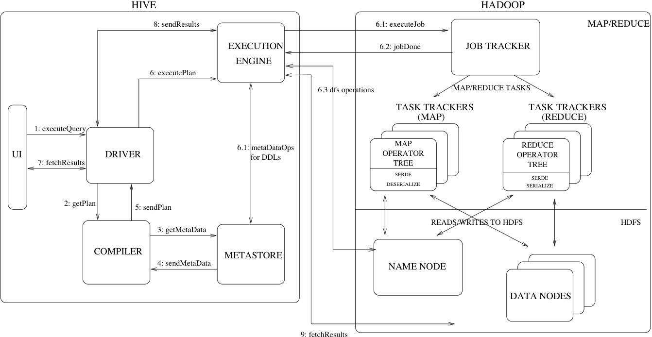
  3. The internal design of Hive is complex but clear. Every component has very distinctive jobs to do and decouples user interface from the coordination, compilation and execution. There is a picture of the design of Apache Hive at the end of this review, which I found very helpful. As I pointed out, the execution flow is very easy to understand.

Weak points:

  1. Hive was originally planned back in 2007 and got open sourced in 2008, so Hadoop MapReduce is pretty much the only choice as execution engine for Hive. It’s definitely one of the main drawbacks of Hive from today’s point of view since Hadoop is much slower than other distributed execution engine like Spark. Replacing Hadoop with Spark or something else would make Hive much faster. I’ve seen some works about Hive on Spark or Spark SQL, and the latter one is claimed to be 100 times faster than original Hive according to Is Apache Spark going to replace Hadoop.
  2. I personally prefer the control flow language like Pig Latin over declarative query language like HiveQL. Programmers can use control flow language to achieve and organize complex nested logic and hence better for extracting more information from data. Pig scripts are also easy to optimize and efficient comparing to SQL-like code. Even from the SQL’s standard, Hive is not complete considering that it doesn’t have update, delete or row level insert operations.
  3. Hive could be bad for small data set because of many reasons: MapReduce is a batch-oriented execution model and has long start overhead; Hive itself need to compile the code into executable MapReduce jobs; the distributed storage underneath (HDFS) add another layer of latency. So overall the system has lots of overhead and cannot run small queries efficiently.


Picture from Design – Apache Hive